Chapter 3: Feature Detection

The first step is what the SfM theorem is actually based on. It has to solve a problem: Recognise the 3D shape of an object that is shown in multiple images from different directions. SfM software uses multiple 2D digital images to calculate the precise location of the camera positions from which the images were captured, which can then be used to triangulate the precise 3D position of individual pixels captured in multiple overlapping frames. The SfM software is based on algorithms that first identify individual edges, boundaries or key pixels (called features) within multiple photographs taken while moving around the object or view being recorded. These individual points or pixels, identified in a minimum of three images, are used to create a Sparse Point Cloud of the key points, and these are used to triangulate the precise camera positions (Powlesland 2016: 21). This is called Feature Detection. Without the features, the images cannot be matched and therefore no reconstruction can take place. There are many different approaches to this, but at the moment the most popular is an algorithm called Scale-invariant Feature Transform (SIFT) (Lowe 1999: 2004).

The SIFT algorithm works in several steps. SIFT allows the relative position of the feature to shift dramatically with only small changes in the descriptor (Carrivick/Smith/Quincey 2016: 40). A descriptor is a unique code that can describe a feature in an image in a way that is independent of orientation or illumination. It is therefore able to recognise individual features and also find them in other photographs, because each feature is given the same descriptor in every photograph, regardless of orientation or lighting conditions. This is also why SfM works best with high contrast objects.

Once the features have been detected in a set of photos, the SIFT algorithm looks for partners and discards those features that have none or too few. There are different approaches to this problem, but basically it ends up with a list of matching features in a set of given photos.

Starting the process

This is how Metashape looks like swhen started.

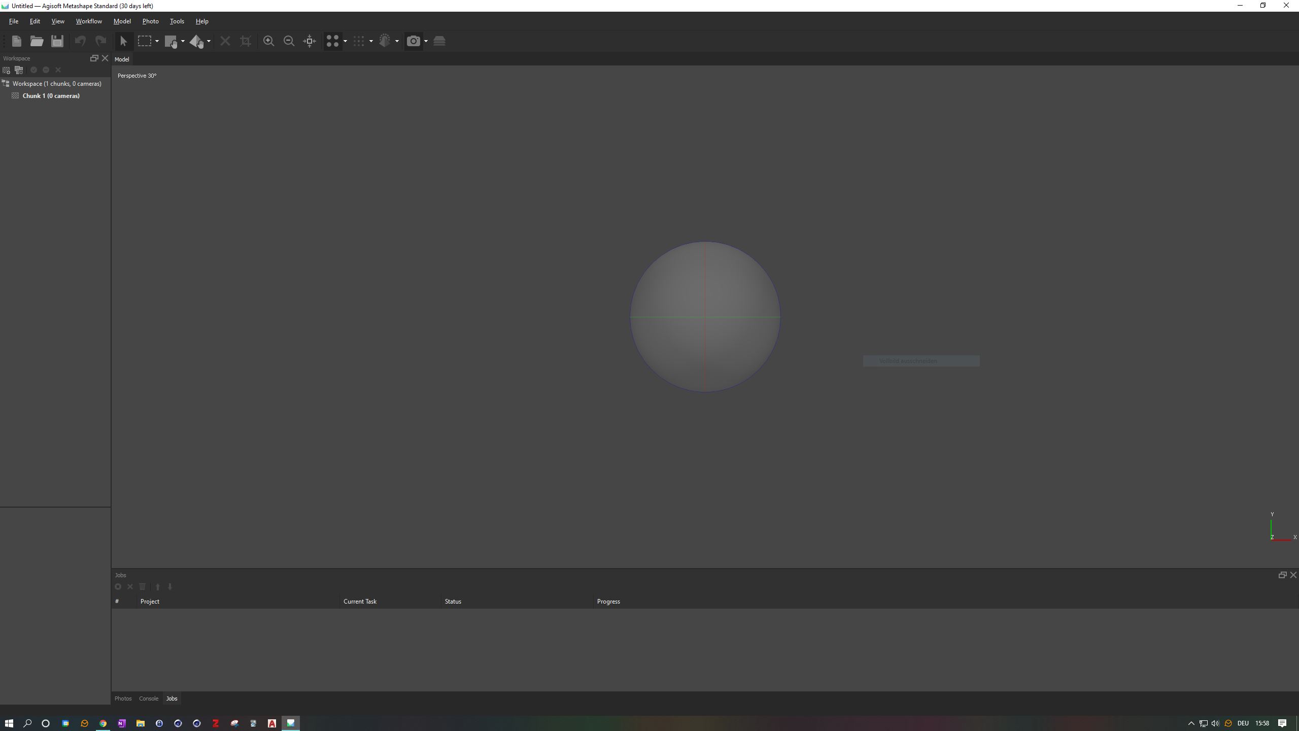
First you need to start the application, which you can find in the Start menu/Agisoft, where you should find the executable Agisoft Metashape Standard (64 bit) (or similar). Once the software has started, you'll see an empty Workspace on the left, the grey Perspective Model View on the right and Tools at the top of the screen. To add your colour corrected photos, press the Add Photo-Button at the top of your workspace or go to the Workflow menu and click on Add Photos=. A file dialog will appear where you can navigate to your data set. Select all the images in this folder at once by clicking on them and pressing CTRL+A/STRG+A. Open the images by clicking on the Open button. You'll see three tabs at the bottom of the screen: Photos, Console, Jobs. Click on Photos. You should now see the opened pictures at the bottom of your screen.

Aligning

Here, you'll find the Align Photos... command.

We will now start the alignment process. Please open the Workflow menu at the top and select Align Photos.... A settings box will appear. For this example, we will use High Accuracy and Generic Pair Preselection. Press the OK button and let the computer do all the work.

Additional information: High Accuracy means that the software will process the photos in their original resolution. Medium Accuracy will downscale the photos by a factor of 4, Low by a factor of 16 and Lowest by a factor of 64. On the other hand, Highest Accuracy will upscale the image by a factor of 4. This is only recommended for very sharp and professional images. Of course, the higher the accuracy, the longer the calculation time. In Generic Preselection, the software will first pre-align the photos at the lowest accuracy setting and then look for common features in the already roughly aligned photos. In Reference Preselection/Sequential, the software will only search for features in adjacent photos, rather than in each photo. This is particularly useful if you have taken the photos sequentially.

Rotating and cleaning the Sparse Point Cloud

After alignment, the result should look something like this.

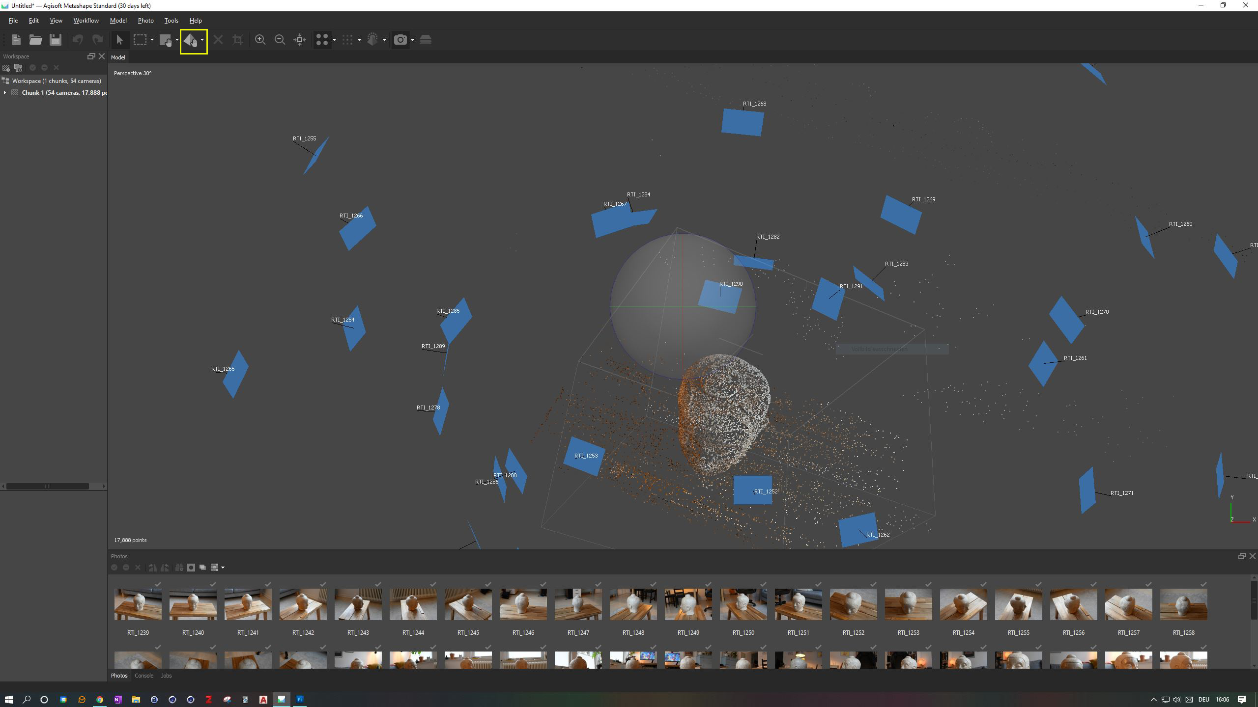
The result of the first alignment step should look something like this. As we are working with a non-referenced coordinate system, the model is somewhere in virtual space. We will first try to move it to the centre of the screen and orient it correctly. To do this, we first want to get rid of these blue boxes. The blue boxes represent the positions where the photos were taken. To remove them, click on the small Camera Icon in the top menu. To move the object, use the Move tools from the top menu and the mouse wheel to zoom. You can also use the mouse wheel to move the object. Use the Navigation tool to move your view and the Move Object tool to move the object to the centre of the world. You can rotate around the object by clicking on the rotation sphere in the centre of the screen. Try to move the object inside this sphere, as you can see in the last screenshot. If you position your object correctly, it will be much easier to navigate around it when you adjust the bounding box.

Cleaning unnecessary points

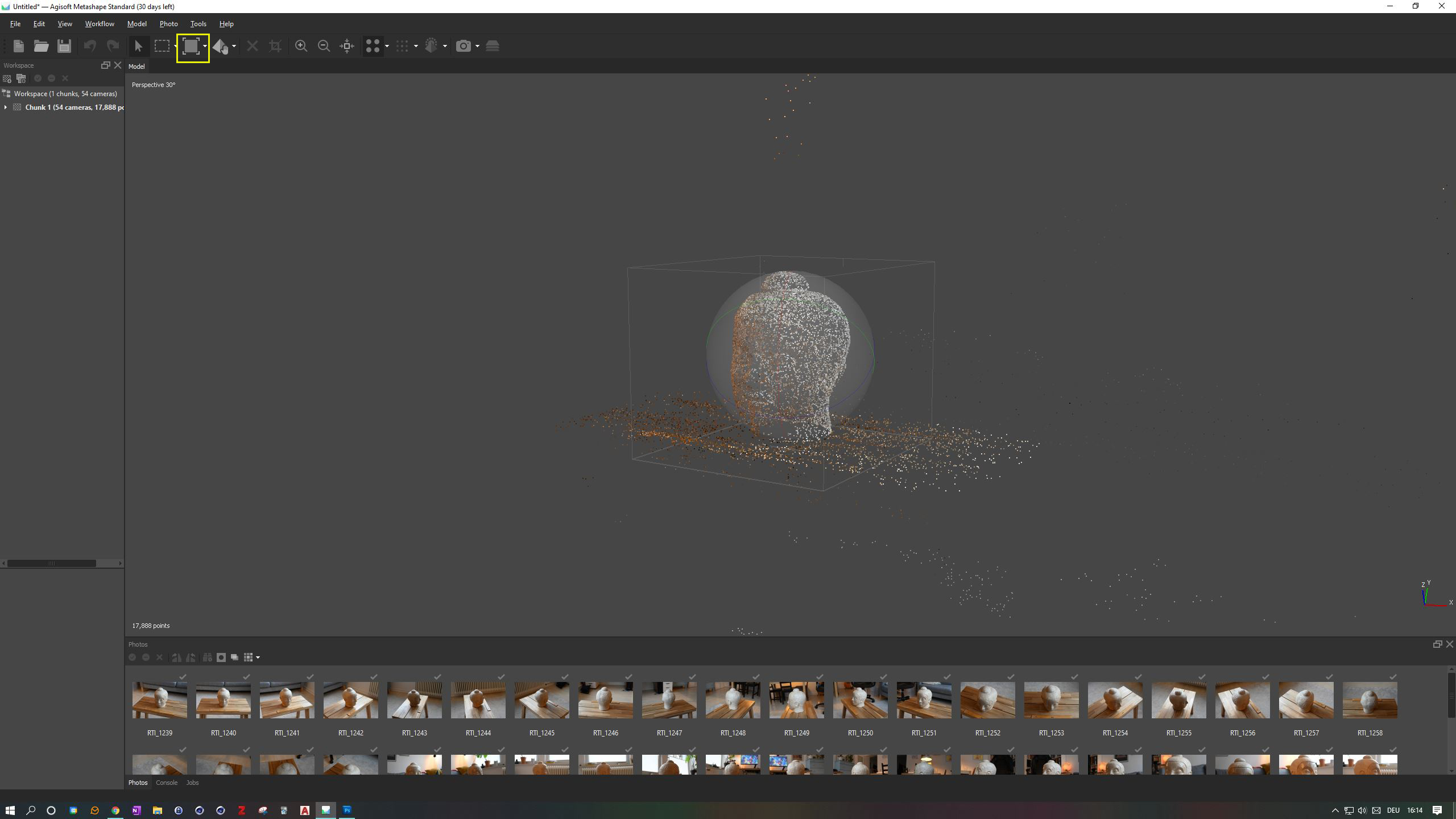
If you zoom out a bit, you will see a lot of points in the background that we no longer need. We can either select and delete them by hand, or we can simply adjust our Bounding Box around the object. Only points inside the bounding box will be processed. You should have already seen the box around the object, as Metashape automatically tries to estimate the object of interest. We still need to make sure that all the necessary points are inside this box, which also includes parts of the table where we have placed our scale. Try to navigate around the object to see it from all sides and use the Move, Resize and Rotate Region tools to adjust the box around the object (and the scale!). Make it as small as possible without compromising parts of the object. The result of the cleaning and positioning should look like this. Don't worry if it doesn't look exactly like the picture here, but try to get as close as possible.

Bibliography

- Carrivick, Jonathan L., Mark W. Smith, und Duncan J. Quincey. 2016. Structure from Motion in the Geosciences. Chichester: Wiley Blackwell.
- Powlesland, Dominic 2016: “3Di - Enhancing the Record, Extending the Returns, 3D Imaging from Free Range Photography and Its Application during Excavation.” In: The Three Dimensions of Archaeology. Proceedings of the XVII UISPP World Congress (1–7 September 2014, Burgos, Spain), edited by Hans Kamermans, Wieke de Neef, Chiara Piccoli, Axel G. Posluschny, and Roberto Scopigno, 13–32. Volume 7/Sessions A4b and A12. Oxford: Archaeopress.
- Lowe, David G. 1999. „Object Recognition from Local Scale-Invariant Features“. In Proceedings of the International Conference on Computer Vision, Corfu (Sept. 1999), 1–8.
- Lowe, David G. 2004. „Distinctive Image Features from Scale-Invariant Keypoints“. International Journal of Computer Vision, 1–28.